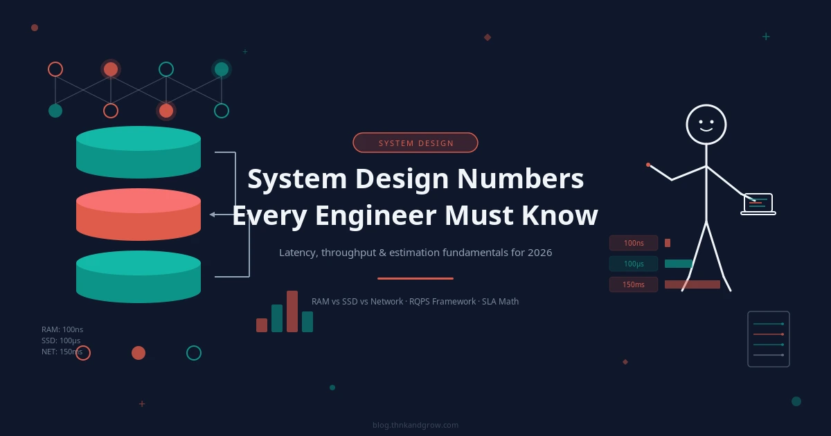
System Design Numbers Every Engineer Must Know in 2026

Picture this: You’re sitting in a system design interview at a top tech company. The interviewer leans forward and asks, “So, how many servers would we need to handle this?” The room goes quiet. Your mind races. You know the architecture — microservices, caching layer, message queue — but the actual numbers? Gone. You freeze.

This scenario plays out every day in interview rooms from Ho Chi Minh City to Singapore, and in architecture meetings at companies across Southeast Asia. The difference between the engineer who answers confidently and the one who stumbles isn’t raw intelligence or years of experience. It’s a set of foundational numbers — internalized, ready to deploy — and a repeatable framework for using them.

In 2026, as distributed systems grow more complex and infrastructure decisions carry real financial weight, back-of-the-envelope estimation has become a non-negotiable core skill. Whether you’re preparing for a Staff Engineer interview at Google, making architectural decisions at a Vietnamese fintech startup, or helping your CTO justify infrastructure spend, these numbers are your foundation. Let’s build it.

Why These Numbers Matter More Than Ever

System design interviews at top-tier companies — Google, Meta, Amazon, Netflix — explicitly test estimation skills at the Senior and Staff Engineer level. It’s not enough to draw boxes and arrows on a whiteboard. Interviewers want to see you reason quantitatively about your design choices.

But the value extends far beyond interviews. In day-to-day engineering work, these numbers allow you to make fast, confident architectural decisions without needing to run actual benchmarks. Should you add a caching layer? The answer lives in your latency table. Can your PostgreSQL instance handle the projected read load? Your throughput benchmarks tell you before you write a single line of code.

Knowing these numbers also prevents two expensive failure modes:

• Over-engineering: Building a distributed, horizontally-scaled system for 1,000 users — wasting months of engineering time and thousands of dollars in infrastructure costs.
• Under-engineering: Launching a monolith for a product that hits 100 million users in six months, then scrambling to rebuild it under production load.

Finally, when you need to communicate infrastructure costs to a CTO or a non-technical stakeholder, credible estimation — grounded in real numbers — makes the difference between a convincing proposal and hand-waving.

Latency Numbers: The Speed Hierarchy You Must Memorize

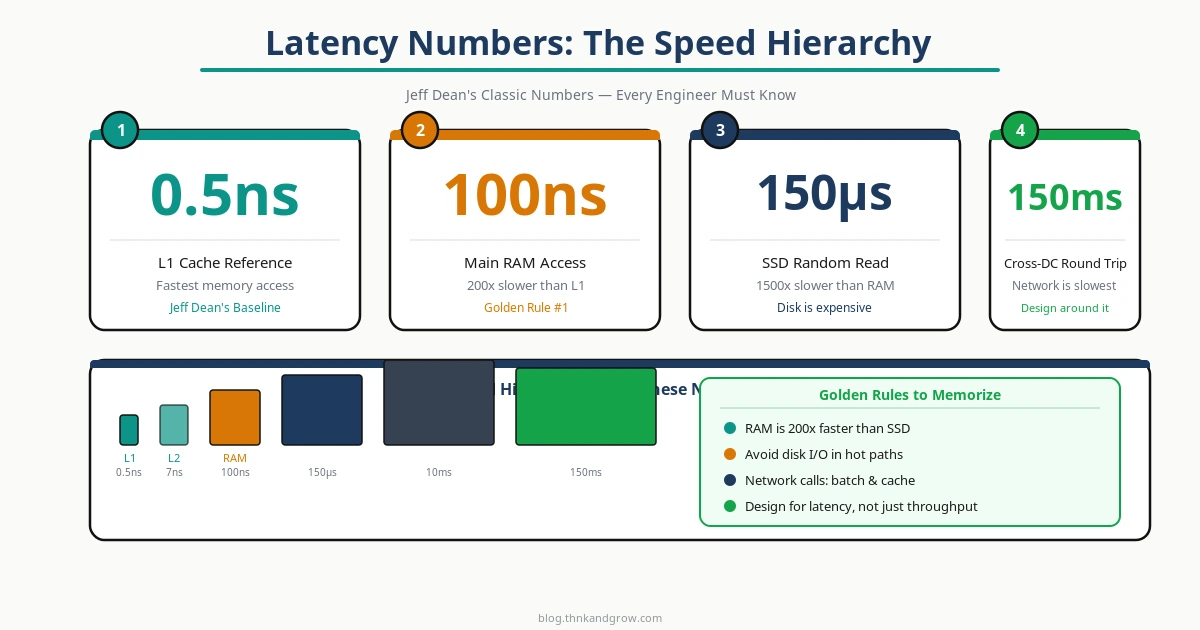
Every system design conversation ultimately traces back to latency. The canonical reference is the latency table originally compiled by Jeff Dean, Google Fellow, and Peter Norvig. Updated periodically to reflect hardware improvements, this table is the single most important reference in system design.

Here are the numbers you need to know cold:

L1 cache reference              ~0.5 ns
L2 cache reference              ~7 ns
Main memory (RAM) reference     ~100 ns
Read 4KB randomly from SSD      ~150 µs
Round trip within datacenter    ~0.5 ms
Read 1MB sequentially from HDD  ~2 ms
Disk seek (HDD)                 ~10 ms
Cross-continent round trip      ~150 ms

The golden ratios to burn into memory:

• RAM is ~1,000x faster than SSD
• SSD is ~10x faster than HDD
• Intra-datacenter network: ~0.5ms
• Cross-continent (e.g., Singapore → Europe): ~150ms

Why do these matter architecturally? Consider a simple question: “Should we cache this database query?” If your query hits PostgreSQL on SSD (~150µs) but your users in Hanoi are hitting a server in Singapore (adding ~30-50ms of network latency), the database read is barely a rounding error. But if you’re making that database call synchronously on every request, and you’re doing it 50 times per page load, suddenly you’re looking at 7.5 seconds of pure database wait time. Caching drops that to nanoseconds.

Similarly, the question “Can we afford a synchronous cross-region call?” almost always answers itself once you internalize that cross-continent latency is 150ms. That’s your entire latency budget for a responsive user experience, gone in one network hop.

Powers of Two: Your Mental Math Shortcut for Storage

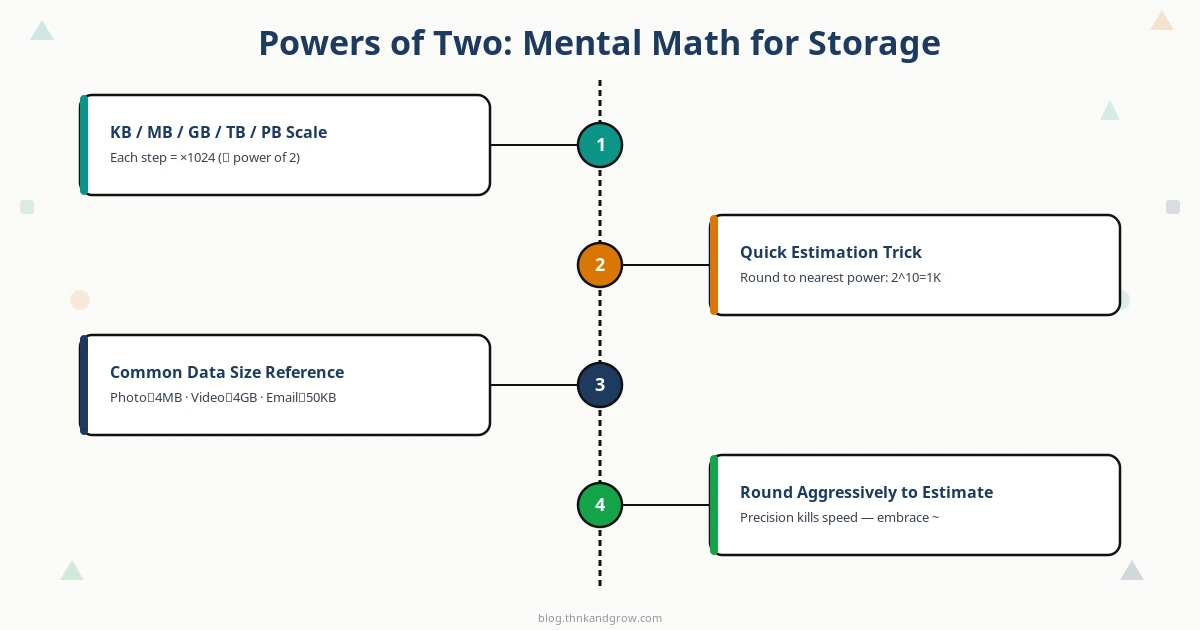
Storage estimation is arithmetic, and the powers of two are your calculator:

2^10  =  1,024        ≈  1 KB  (1 thousand bytes)
2^20  =  1,048,576    ≈  1 MB  (1 million bytes)
2^30  ≈  1 billion    ≈  1 GB
2^40  ≈  1 trillion   ≈  1 TB
2^50  ≈  1 quadrillion ≈ 1 PB

Pair these with common data type sizes:

• Integer (int32): 4 bytes
• Long / Timestamp: 8 bytes
• UUID: 16 bytes
• Average tweet / short text record: ~300 bytes
• Average image: ~300 KB
• HD video per minute: ~100 MB

Now you can estimate storage in seconds. Example: A Twitter-like app with 10 million daily active users, each posting 1 tweet per day:

10,000,000 users × 300 bytes = 3,000,000,000 bytes = ~3 GB/day

Over 5 years: 3 GB × 365 × 5 = ~5.5 TB. That’s a single well-provisioned database server, not a distributed storage cluster. The numbers tell you what to build.

The critical discipline here: round aggressively. Precision is the enemy of speed in estimation. Use 10M instead of 9.7M. Use 300 bytes instead of 287. You’re aiming for the right order of magnitude, not the right answer to three decimal places.

Availability Numbers: Understanding the “Nines”

When a product manager says “we need five nines of availability,” do you know what that actually means in practice? Here’s the SLA table:

99%      → 3.65 days downtime/year
99.9%    → 8.77 hours downtime/year
99.99%   → 52.6 minutes downtime/year
99.999%  → 5.26 minutes downtime/year

The jump from 99.9% to 99.999% is not incremental — it’s a fundamentally different engineering problem, requiring active-active multi-region deployments, automated failover, and often a 10x increase in infrastructure cost.

Here’s the insight most engineers miss: availability is multiplicative, not additive. If your API service has 99.9% availability and your database has 99.9% availability, your system’s availability is not 99.9%. It’s:

99.9% × 99.9% = 99.8%

Every component you chain in series reduces your overall availability. This is why microservices architectures require careful SLA management — ten services each at 99.9% gives you a system availability of roughly 99%, which is 3.65 days of downtime per year.

Redundancy is the fix, and the formula is: Availability = 1 - (1 - p)^n, where p is the availability of a single component and n is the number of redundant instances. Two instances at 99.9% gives you: 1 - (0.001)^2 = 99.9999%. Redundancy is powerful — but it has a cost, and that cost must be justified by actual business requirements.

Throughput Benchmarks: Know Your Components’ Limits

Before you select a technology, you should know roughly what it can handle. These are ballpark figures for well-configured, single-server deployments:

Nginx (HTTP server)     ~50,000 – 100,000 req/s
PostgreSQL              ~5,000 – 15,000 queries/s
MySQL                   ~10,000 – 30,000 queries/s
Redis                   ~100,000 – 1,000,000 ops/s
Kafka                   ~1,000,000 messages/s per broker
MongoDB                 ~20,000 – 80,000 ops/s
Memcached               ~200,000 – 1,000,000 ops/s

These numbers directly guide technology selection. If your system needs to handle 200,000 read operations per second on user session data, PostgreSQL simply cannot do it on a single node — but Redis handles it comfortably. That’s not a preference; it’s arithmetic.

Two important caveats: First, these numbers shift significantly based on hardware, query complexity, network conditions, and configuration. A complex PostgreSQL JOIN with no indexes might perform 100x worse than the benchmark above. Second, always add a 2-3x safety buffer when planning capacity. Real production traffic is spiky, unpredictable, and unkind to engineers who plan for average load.

The RQPS Framework: A Step-by-Step Estimation Method

Knowing individual numbers is necessary but not sufficient. You need a repeatable framework to combine them into a coherent estimate. The RQPS framework — Requirements → QPS → Storage → Bandwidth → Servers — gives you exactly that.

Step 1: Clarify Requirements

Before calculating anything, nail down: DAU (Daily Active Users), read/write ratio, and data retention period. Wrong assumptions here cascade into wildly wrong estimates downstream.

Step 2: QPS Estimation

QPS = DAU × requests_per_user_per_day ÷ 86,400

Peak QPS = QPS × 2 to 3  (traffic spike multiplier)

Step 3: Storage Estimation

Daily storage = DAU × writes_per_user × data_size_per_write
Total storage = Daily storage × retention_years × 365

Step 4: Bandwidth Estimation

Incoming = Write QPS × request size
Outgoing = Read QPS × response size

Step 5: Server and Cache Estimation

Servers needed = Peak QPS ÷ QPS per server
Cache size = hot data volume × cache hit ratio target

Putting It All Together: A Worked Example

Let’s design the backend for a Twitter-like feed system targeting 10 million DAU in Southeast Asia — think a product competing with X in the Vietnamese or Indonesian market.

Assumptions: Each user posts 1 tweet/day, reads 50 tweets/day. Read/write ratio: 50:1. Tweet size: 300 bytes. Retention: 5 years.

QPS

Write QPS = 10M × 1 ÷ 86,400 ≈ 116 writes/s
Read QPS  = 10M × 50 ÷ 86,400 ≈ 5,800 reads/s
Peak Read QPS ≈ 5,800 × 2 = ~11,600 reads/s

Storage

Daily: 10M × 300 bytes = 3 GB/day
5-year total: 3 GB × 365 × 5 ≈ 5.5 TB

Bandwidth

Incoming: 116 × 300 bytes ≈ 35 KB/s  (negligible)
Outgoing: 5,800 × 300 bytes ≈ 1.74 MB/s

Servers

Read servers: 11,600 ÷ 5,000 (PostgreSQL) ≈ 3 servers + replicas
Or: 11,600 ÷ 100,000 (Redis) = 1 cache server handles it entirely

What do these numbers reveal? At 11,600 peak read QPS, a caching layer with Redis is not optional — it’s the entire architecture. A single Redis node handles the read load. PostgreSQL handles writes and serves as the source of truth. You need a CDN for any media. Read replicas become necessary only if cache miss rates are high. This analysis took under 10 minutes, and it produced real architectural decisions.

Common Mistakes and How to Avoid Them

• Being too precise: Spending five minutes calculating 9,722,341 users instead of rounding to 10M wastes time and signals poor judgment. Estimation is about order of magnitude.
• Forgetting peak traffic multipliers: Average QPS is not design QPS. Traffic spikes during Tết, product launches, or viral moments can be 3-5x your daily average.
• Ignoring availability multiplication: Two 99.9% services give you 99.8%, not 99.9%. Always multiply, never average.
• Using outdated numbers: NVMe SSDs, modern CPUs, and network hardware improve constantly. Sanity-check your reference table annually.
• Skipping the clarification step: Estimating without confirming DAU, read/write ratio, and retention period is like navigating without a destination. The math will be internally consistent and completely wrong.

Conclusion: Make Estimation a Core Engineering Habit

The numbers in this article are not interview trivia. They are the mental models that separate engineers who build systems that scale gracefully from those who discover bottlenecks in production at 2am on a Friday. The engineer who can say, confidently, “At 10 million DAU with a 50:1 read/write ratio, we’re looking at roughly 12,000 peak read QPS — PostgreSQL won’t cut it without a Redis caching layer” is not showing off. They are doing their job at the highest level.

Internalize the latency table until the ratios feel instinctive. Practice the RQPS framework on real systems weekly — not just when you have an interview coming up. Treat estimation as a core engineering competency, the same way you treat code quality or system reliability.

Here’s your call to action: Pick a system you use every day — YouTube, Shopee, Grab, or Zalo — and run it through the RQPS framework right now. Estimate the DAU, guess the read/write ratio, calculate the QPS, and see what architecture the numbers suggest. You’ll be surprised how quickly the fog lifts, and how much more confidently you’ll approach your next design conversation — whether it’s in an interview room or a product architecture meeting.

The numbers are learnable. The framework is repeatable. The skill is yours to build.